| 3.5 Wave shaping | ||
|---|---|---|
| Chapter 3. Audio | | |
| 3.5 Wave shaping | ||
|---|---|---|
| Chapter 3. Audio | | |
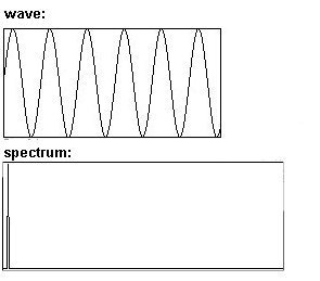
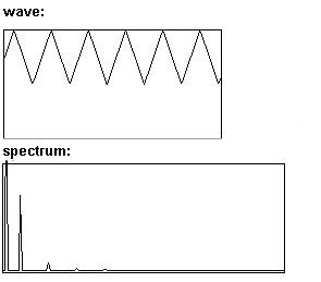
In 3.1.1.1.2 you learned about different waveforms (sine, sawtooth, triangle, square, and pulse). Pd has objects for two of these, namely "osc~" for sine waves and "phasor~" for sawtooth. You can use an array to display the waveforms:
patches/3-5-1-1-waveform-graph.pd
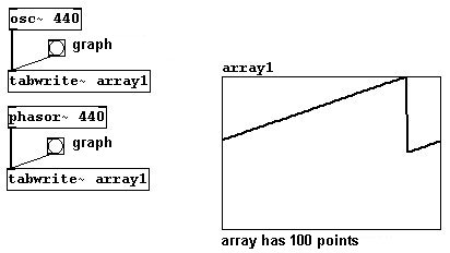
N.B.: The sawtooth of the "phasor~" object always goes from 0 to 1; it never goes into the negative range. You could make it stronger, however, by performing a small calculation:
patches/3-5-1-1-strong-phasor.pd

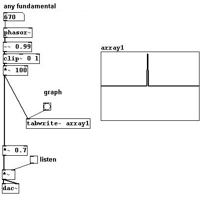
You can also create other waveforms by attaching a few operations to "phasor~". To accomplish this, you'll need to use a new object: "clip~", which cuts off everything outside the indicated range. As the arguments, enter two numbers for the lower and upper limits; numbers outside of these limits will be 'clipped':
patches/3-5-1-1-other-waveforms.pd

Now on to the Triangle wave:

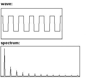
Square wave:
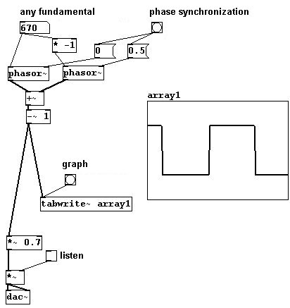
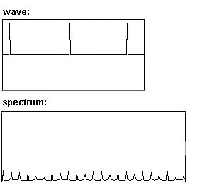
Pulse:
These are all standard waveforms that exhibit certain characteristics:
Sine: a single ton without any overtones
Triangle: like a sine wave, except with the odd partials as well
Square: only the odd partials
Sawtooth: all partials

Pulse: all partials present at nearly equal intensities
You can observe that symmetrical waveforms exhibit only the odd partials (within each period, exactly two periods of each subsequent odd partial fit; that's what is meant by symmetrical), while asymmetrical waveforms always exhibit the even partials as well.
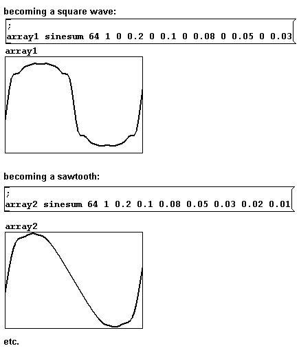
These waveforms can also be approximated using additive synthesis:
patches/3-5-1-1-waveform-fourier.pd
There is unlimited room for experimentation here and that's one way to arrive at new sounds. You can also draw your own waveforms directly in an array. To do this, you must be in execute mode and move the mouse to a line in the array. The cursor arrow changes direction:
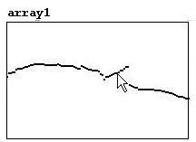
While holding the mouse button, move the mouse to draw your own waveform.
This is, however, somewhat tedious and 'inelegant'. Let's examine then the theory of 'wave shaping':
A linear function undergoes what's called a "transfer function". For linear functions, you can use the "phasor~", which always goes from 0 to 1. You could make a cosine wave, for example, using the "cos~" object, which calculates a cosine function:

You can make all kinds of transfers this way; here's another example:
patches/3-5-1-2-transferfunction.pd

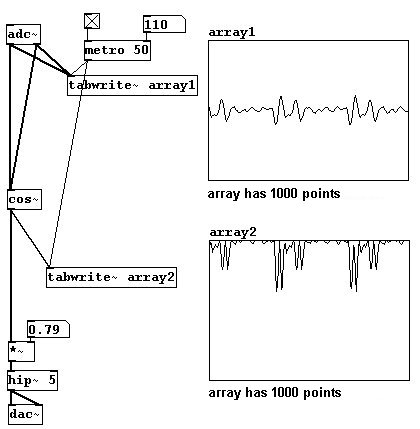
You could also record noise into an array and then read it out periodically - i.e., read the same thing out again and again (cf. Karplus-Strong). If you do this more than 20 times a second, you'll hear a pitch:

The spectrum of this sound is naturally somewhat unpredictable. Every time you fill the array with random numbers with the "noise~" object, you get a new wave with new characteristics.
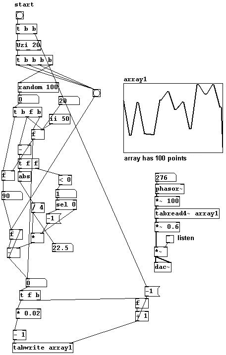
But there is still somewhat of a system at work. You could, for example, interpolate all the clicks (large jumps in the waveform) to achieve a smoother resultant waveform. Let's generate random points using linear interpolation ("Uzi" (Pd-extended) generates the number of bangs specified in its argument and sends them as fast as possible):
The result will be even softer if you use a sinusoid interpolation instead of a linear one. Here, ten points are used for interpolations:
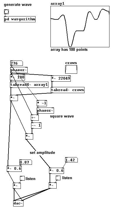
patches/3-5-1-3-wavgorithm+sin.pd

Now the connection from the end of the period to its beginning has to be interpolated as well. We'll use a windowing for this and program the calculation in a subpatch.
patches/3-5-1-3-wavgorithm+sin+fenster.pd
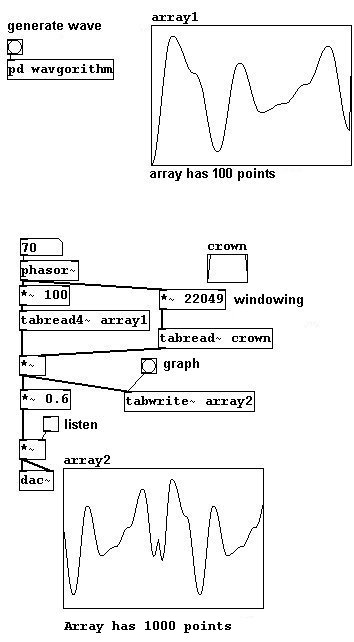
This way, the membrane is at 0 at the beginning and end of each period. The result could be even smoother if it were "windowed" with the Hanning window (3.9.4.1).
In addition, transfer functions using known waveforms - e.g., a square wave, which would intensify the odd partials - are also possible.
And so on. In these last few examples, the wave has to be created on the control level; in contrast to the first examples that used transfer functions, we cannot change these "live".
A final technique that might be considered wave-shaping synthesis is "wave-stealing". This involves taking a small section of known pieces of music...
patches/3-5-1-4-wavestealing.pd

With the following patch, it is possible to record waveforms with a microphone to sing waveforms.
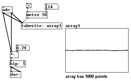
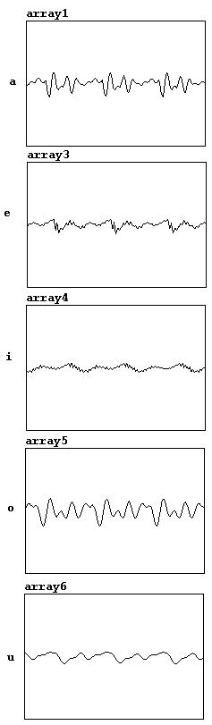
The vowels (German pronunciation) look something like this:
You can also divide a sawtooth wave into even and odd partials. To accomplish this, you'll need to use "wrap~". It calculates the difference between the input number and the nearest integer below it (the absolute value is taken, so that the result is always positive). A few short examples:
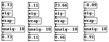
And now for the sawtooth division: the "wrap~" object is used to phase shift the sawtooth wave; this is then added to and subtracted from the original signal, resulting in a sawtooth wave with twice the frequency and a square wave.
patches/3-5-2-3-even-odd-partials.pd

At this point, a particularly thorny problem in digital sound processing must be addressed: foldover. Let's first examine this situation:
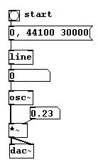
What happens? After 22050 Hz, the direction changes until it reaches 44100 Hz, at which point you get a pitch with a frequency of 0 Hz (after this, the pitch would go up again). The reason for this is that a sample rate with of 44100 Hz can produce a wave of 22050 Hz maximum (cf. 3.1.1.3.1). Moreover, there are some typical reading errors. Let's take a look at three waves with different frequencies: the top has a frequency of 11025 Hz, the middle 22050, and the bottom somewhat more than 22050. The markings stand for reference points (for the samples), which have a constant speed of 44100 per second.
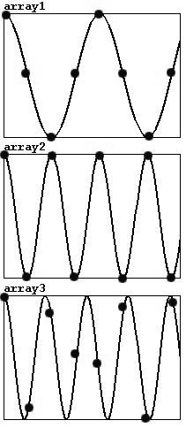
Each period in a wave with 11025 Hz can be represented with four points (of course, the characteristic sine wave shape is lost). 22050 Hz is the highest frequency that can be correctly represented, since Nyquist's Theorem requires at least two points per period. Errors will occur with frequencies higher than this; not every period will be captured and the points of measurement will actually record a lower frequency instead of a higher one.
The problem is much more pronounced for waveforms that exhibit overtones, e.g., with a pulse:
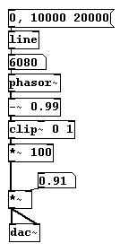
Here the effect can be noticed much earlier: after 700 Hz some overtones are inaccurately captured. This is because the pulse waveform practically consists of just a single line, which is quickly 'missed'. A solution to this problem is to begin with a pulse waveform, but to broaden the wave as the frequency increases, so that you end up with a sine wave at the end: