| Chapter 3. Audio | ||
|---|---|---|
| | ||
| Chapter 3. Audio | ||
|---|---|---|
| | ||
Table of Contents
From here on out, large patches are pre-assembled in additional files (http://www.kreidler-net.de/pd/patches/patches.zip).
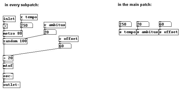
Many of the functions described in Chapter 2 will not be used in the rest of the text - e.g., the "send" and "receive" objects - although they are certainly often used in practice. The patches you'll encounter here have been reduced to the bare essentials. However, when you actually use the techniques presented in a composition or performance, it will be necessary to store them as subpatches and connect them with "inlets"/"outlets", etc. You can see one example of this here: 3.4.2.4.
Let's return to our first example. You heard a tone with a frequency of 440 Hertz (later with other frequencies, other pitches). You could turn it on and off - i.e., adjust the dynamic from loud to inaudibly quiet.
About pitch: Pd works with two kinds of pitches - Hertz or MIDI numbers. The traditional signs: A, B-flat, G-sharp, etc. are not used at all in Pd. Instead all chromatic pitches have MIDI numbers: A4 is the number 69, B-flat4 is 70, etc. The other way to describe pitch in Pd is in Hertz. To understand this, we need to understand a bit about musical acoustics.
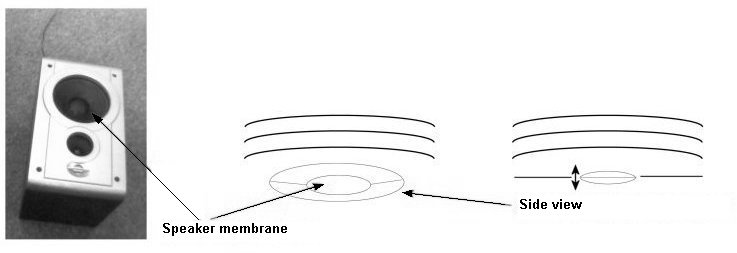
Sound is air in vibration. Traditional instruments are used to vibrate air at specific frequencies. You can do this, e.g., with strings (violin), lips (trumpet), or membranes (timpani). We even have a membrane in our ears - the eardrum - that vibrates sympathetically with vibrations in the air. Our brain transforms these vibrations into a different form, which is what we would call sound.
In electronic music, we use speakers to generate sound. These also have a membrane (or several) that vibrates back and forth, which causes the air to vibrate.
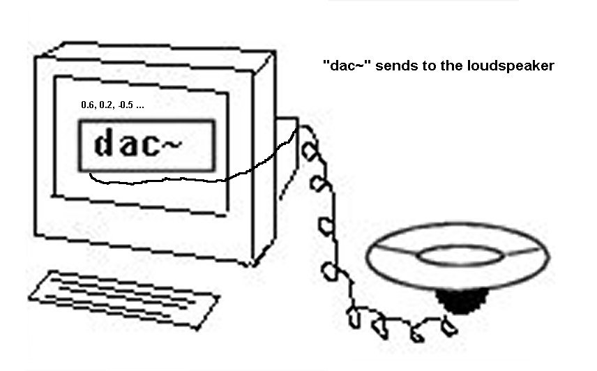
The vibrations of this membrane are controlled by the computer. In Pd, the "dac~" object (digital audio converter) handles this. Here's how it works: sound is a physical phenomenon - vibrations in the air to be precise - and, as such, it is analog. Computers, however, work only with numbers, which means they are digital. The "dac~" object turns numbers into sound by converting numbers into fluctuations of electrical current that - once amplified - cause the speaker membrane(s) to vibrate accordingly.
 |
The reverse of the this process would be to connect a microphone to a computer. A microphone also has a membrane that responds to vibrations in the air and converts these vibrations into fluctuations in electric current, which it sends to the computer where they are then converted into numbers. In Pd, this input can be received with the "adc~" object.
 |
Let's go back to speakers for a moment. A speaker's membrane can move back and forth. The outermost position (the most convex) is understood by the computer as position 1. The innermost position (the most concave) is position -1. When the membrane is precisely in the middle, as when at rest, this is position 0. All other positions are values of between -1 and 1.
 |
In reality, these movements are so small and so fast that they almost cannot be observed with the naked eye.
Let's imagine that a membrane moves from one extreme limit to the next (most convex, most concave) at a constant tempo:

Let's mark the individual stages:

In an abstracted form with membrane position on the y-axis and time on the x-axis, we could represent such motion like this:


In physics terminology, this is called a wave. Here you can clearly see the waveform - a triangle.
There are different waveforms for different kinds of membrane movement. Their names reflect their visual resemblance:
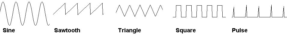
The Pd object "osc~" creates a sine wave.
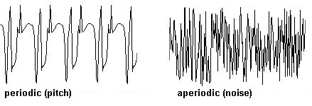
One important thing to remember with regard to waveforms: they repeat constantly without changing their motion characteristics. Vibrations that exhibit this quality are said to be periodic. A period is one complete cycle of a vibration that constantly repeats.

What makes periodic vibrations special is that we hear them as clear tones with definite pitch. In contrast, noises are aperiodic vibrations.
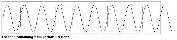
Let's first discuss periodic vibrations. It is possible to simply count the number of periods in a second. This number is a vibration's frequency and is measured in "Hertz" (Hz); frequency in this context always means how often something repeats in one second (expressed mathematically: 1/second).
A tone's frequency determines its pitch. A440 (also called A4, the standard pitch that orchestras use for tuning) means that the air vibrates periodically at a rate of 440 times per second; C5 vibrates 523 times per second; the low G on a cello vibrates about 100 times per second.
Here you can already see: the slower the frequency, the lower the pitch appears to our ear. In fact, humans - depending on age - hear pitches between 20 Hz and 15000 Hz. Children can hear up to 20000 Hz; elderly people can often only hear up to 10000 Hz. Dogs and bats can hear well over 20000 Hz. This range is referred to as ultrasonic. In contrast to this is the infrasonic range, which is lower than the bottom of the audible threshold - i.e., between 0 and 20 Hz. This range is perceived by us as rhythm. You can use Pd to experience this for yourself with the following experiment:
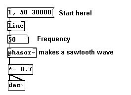
You hear a rhythm of clicks (that's the sound of a sawtooth wave) that gradually gets faster. After a certain speed (over 20 clicks per second), our perception 'shifts gears' and begins to hear a low pitch. For the air (and for the computer), this is still a "rhythm". But for the human ear (ca. 20 Hz) it's a pitch! The faster this rhythm becomes, the higher the pitch we hear.
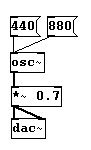
Another defining characteristic of the human ear is that it hears pitches logarithmically. This means when a given frequency is doubled, we perceive this as an octave leap. If you change from A4 (440 Hz) to its double (880 Hz), you hear A5, which is exactly one octave higher:
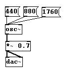
If we want to hear an octave above 880 Hz, we have to double it again. 880 + 880 = 1760:
Just to be clear: from 30 Hz to 60 Hz, we hear an octave but from 1030 Hz to 1060 Hz, we hear just a small step. In fact, the jump from 10000 Hz to 20000 Hz is only an octave!
Another important concept: let's add the same amount to a fundamental frequency, say 100 Hz - which is roughly the frequency of the open G-string on a cello - to which we'll add 100 Hz successively:
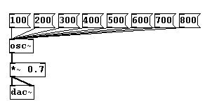
You hear an octave from 100 to 200, a fifth from 200 to 300, a fourth from 300 to 400, etc. In mathematics, this is an additive process in which the same amount is added each time. Our ears, however, perceive that this amount gets smaller and smaller with every step:
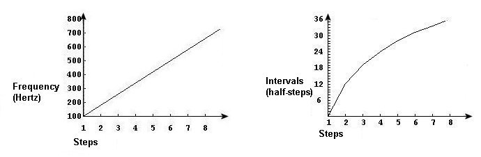
The graph on the left shows the mathematical function - a linear function. The right side shows what we hear - a logarithmic function.
If you want to hear a linear progression - i.e., a process by which the same interval is added, for example the octave - the mathematical function has to be exponential:

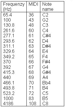
The conversion from linear to logarithmic progressions in Pd is accomplished by using MIDI numbers and frequencies. MIDI numbers reflect the way we hear in that the intervals we hear correspond to an equivalent interval in MIDI numbers: one whole number per half-step. You can convert entries in frequencies and MIDI numbers in Pd:

A small table of MIDI numbers, frequencies, and their traditional names:
N.B.: Oscillators like "osc~" or "phasor~" have to receive their input in Hertz.
One has to remember that for Pd, sound is only numbers. Positions of a speaker's membrane are numbers between -1 and 1.
|
Objects like "osc~" generate a very fast sequence of numbers between -1 and 1 that is sent to the speaker by the "dac~" object. To be specific, 44100 numbers per second are generated and sent. The loudspeaker makes 44100 tiny movements between -1 and 1 within one second. This number, 44100, is called the sample rate.
Every sound in Pd is produced using numbers between -1 and 1 at a rate of 44100 numbers per second (sample rate). A single individual number is called a sample.
All Pd objects that generate or process data at this speed have a tilde "~" in the object box. These objects are connected to each other with thick cables. We call these series of numbers signals.

Whenever you want, you can give the "osc~" object a new frequency as input. The cable for this connection is thin, because the input is not in constant transmission. The "osc~" object's outlet, however, is constantly sending signals, i.e., numbers between -1 and 1, 44100 per second (per second means: Hertz).
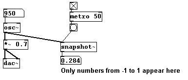
You cannot connect a number box to the "osc~" object's outlet if you want to see the numbers. Number boxes can only be used for control connections, not signal connections. Signal connections are too fast: you wouldn't be able to see 44100 different numbers per second. You can, however, show selected numbers from a signal with the "snapshot~" object. As inputs, it receives the sound signal and a bang that, when clicked, displays the current number when clicked. To see this number, connect either a number box or a "print" object to its output:

If you want a constant stream of these numbers, you could attach a (fast) metronome:
In Pd-extended, you could also use "unsig~", which automatically connects a metronome. Enter the metronome value as the argument:
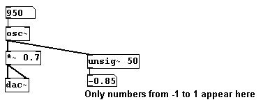
You can also use "sig~" to convert numbers on the control level into numbers on the signal level. You enter a value once into its inlet that is sent out its outlet 44100 times per second.
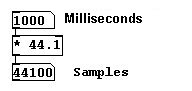
As with frequency (and with amplitude as discussed in the next chapter), there are two different units in Pd for measuring time: samples and milliseconds. Samples are usually used for counting signals while milliseconds are used for control data.
Converting duration in milliseconds to duration in samples:
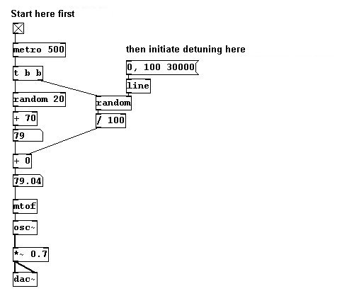
Random MIDI values are gradually offset. (Transition from equal tempered tuning to random tuning):
patches/3-1-1-2-1-random-offset.pd
 |
The number 44100 was chosen for a good reason. As previously mentioned, humans can hear up to 20000 Hertz at most. In 1928, US physicist Harry Nyquist (1889-1976) proposed a theory stating that a frequency of at least twice the signal frequency was necessary to accurately represent a sound signal digitally ("Nyquist-Shannon sampling theorem"). Concretely, this means that one needs the maximum and minimum values for each period to accurately represent a waveform's basic shape, i.e., two points per period:
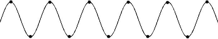
For a wave with 20000 Hz, which equals 20000 periods per second, we need at least 40000 points per second to accurately represent it. To ensure that the entire spectrum of sounds audible to humans was included, a sample rate of 44100 was chosen for audio CDs. This means that waves of up to 22050 Hz could be captured. For computers, a wide selection of frequency bandwidths exist, all the way down to 8000 Hertz for system sounds. High-quality audio recordings work with sample rates of 48000 Hz (48 kHz = kiloHertz, where kilo = thousand), 96 kHz, or even 192 kHz.
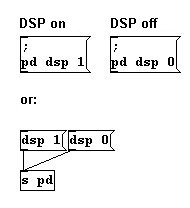
It has become clear that simultaneous processing of numerous signals is very taxing on the computer. Imagine working with 100 "osc~" objects. Each one generates 44100 numbers per second and these have to be synchronized with each other. That's why Pd offers you the option of turning off DSP (digital signal processing) in the main window. This will spare your processor unnecessary work.
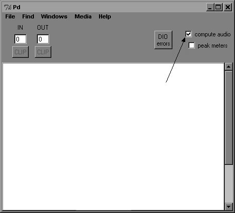
You can also send this as a command; the recipient "pd" is in this case the program itself:
With regard to computer music, the faster the processor, the higher the performance.
Pd lightens its workload by working with samples in blocks rather than individually. This greatly improves performance. The standard block size is 64 samples, but this setting can be changed. More on this at 3.8.1.1
It was previously stated that "dac~" sends the numbers generated by Pd to the speaker membrane (3.1.1.1.1), but this is of course a bit oversimplified. Strictly speaking, the computer's sound card converts the numbers into an electrical current with variable voltage ("digital-analog-conversion" or "da-conversion"); the membrane position is in turn determined by the amount of voltage. Going the other way, membrane fluctuations in a microphone are converted into a variable current, which is then digitized by the computer's sound card.
Sound waves, in contrast to water waves, are longitudinal. Longitudinal waves, also called compression waves, are characterized by the fact that they vibrate along their direction of movement. (Transverse waves, on the other hand, vibrate along an axis perpendicular to the direction of movement.) For further explanation, please consult a high school physics textbook.
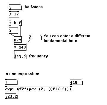
The "mtof" object converts MIDI numbers to frequencies. The formula for this calculation is:


To calculate the frequency of a pitch in equal temperament that is a certain distance away from a given frequency, use this formula:
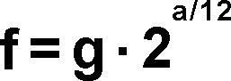 |
'f' is the frequency you want to know, 'g' the frequency of the given pitch, 'a' the interval in half-steps.
For instance, if you want to calculate the frequency of C5 and know that A4 has a frequency of 440 Hz:
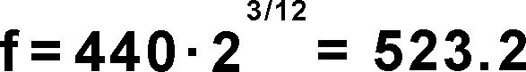 |
In Pd:
For the inverse operation - converting a frequency into MIDI - the formula is:

However, in Pd we have only the natural logarithm based on Euler's number (the mathematic constant 'e'); so we need this formula as well:
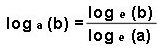
Programmed in Pd:

We've covered the fact that noises are not periodic. You could, however, imagine a noise that lasts 10 seconds and then repeats precisely as before. Such a noise would theoretically have a periodic frequency of 0.1 Hz. So a noise can be more precisely defined as a sound that is aperiodic or has a period of less than 20 Hz. Furthermore, one could also say that the frequencies of noise may have a common fundamental tone that is lower than 20 Hz.
Many exciting experiments have been conducted in the field of acoustics, for example involving the Doppler effect or calculating the length of sound waves. Please consult leading acoustics textbooks for more information.
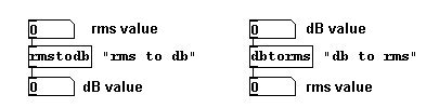
The next parameter of a sound we'll look at is its volume. Traditionally, volume in music is notated using dynamic markings like pianissimo, piano, mezzoforte, etc. Their use is subjective and variable depending on the instrument. In physics, which is what Pd uses as a model for this parameter, volume is represented with objective values in deciBel or root mean square values. Both units are comparable to MIDI numbers and frequencies for pitches. DeciBel (dB) reflect what we hear, where an 'octave' in volume corresponds to 6 dB. The scale ranges from 0 to 130 dB - where a value of between 15 and 20 dB is absolute silence and anything over 120 dB is capable of causing serious hearing damage. After 130 dB we perceive sound only as pain. Root mean square values (rms), like frequencies, do not correspond to what we hear, but are logarithmic values between 0 and 1, where 0 corresponds to 0 dB and 1 to 100 dB. rms refers to the geometric mean calculated from a series of amplitude values. These numbers are first squared, then the average is taken (by adding all values and dividing by the number of elements), and then the square root of this average is taken. The rms value for an audio signal is first calculated using a portion of the audio signal that lasts specific duration; for a heavily fluctuating signal like a pitch frequency, it gives you an idea of the average signal amplitude. The following objects can be used to convert from one to the other in Pd:
The volume of a vibration is determined by its amplitude, which is the degree to which the membrane is displaced outwards or inwards with respect to the neutral position at rest (the zero position). The greater the membrane's movement, the louder we perceive a sound to be. A representation on an axis looks like this:
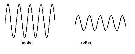
It cannot be emphasized enough: until this is sent to the speaker with the help of the "dac~" object, Pd works only with numbers. If a sound is quiet, this means that the numbers do not span the full range from -1 to 1, but are instead confined to a more restricted range around the zero position, say, between -0.5 and 0.5. This can be accomplished in a patch by multiplying the numbers generated by the "osc~" object by a certain factor:
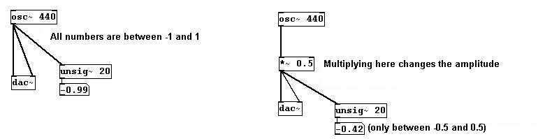
You can use this method to set the volume to any level from absolute silence to as loud as possible (which depends on the speakers and the amplifier you're using, of course).

You could also attach a slider using HSlider (Put HSlider) and setting its range from 0 to 1 (cf. Chapter 2.2.2.3.2 and 2.2.4.3.4):
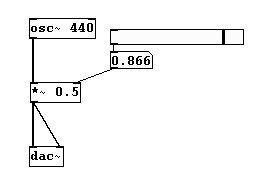
However, moving this slider quickly will result in disruptive sounds. This is because a signal (calculated in samples) clashes with control processing (calculated in milliseconds). If this is only a matter of a few numbers as previously with the factors 0, 0.1, 0.4, 0.7, and 1, this is irrelevant, but beyond a certain speed this can play a significant role. To avoid this problem, you have to replace the control connection with a signal pendant. Use the "sig~" object to convert:
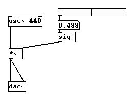
This ensures that the numbers generated by the oscillator (44100 numbers/sec) and those generated by the factor ("sig~" converts them into exactly 44100 numbers/sec) are synchronized. N.B.: if a signal is attached to the "*~" object's right inlet, the object must not have an argument: if you were to enter an argument (like 0.5, as used previously) the object would assume that its right input was control data.
To create a crescendo or a decrescendo, you have to use "line~":
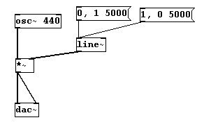
Here's an elegant way to use a slider as a volume regulator ("Potentiometer"):
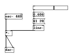
This executes a small crescendo/decrescendo between every step. Filling in steps with intermediate values in this way is called "interpolation" (as already seen with pitches in Chapter 2.2.3.2.3).
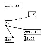
You can calculate the volume of a given sound using "env~", which gives the volume in dB as output. You must always define a span of time in which this average value is to be calculated; its argument is given in samples (this number is usually a power of 2):
The conversion into rms ...
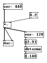
... makes it clear that factors between 0 and 1 are not to be confused with rms values between 0 and 1.
As already mentioned, humans' aural perceptions of volume and pitch do not correspond with the measurements in physics (as observed in the paired diagrams for pitches by frequency and interval). A simple trick for creating a more linear crescendo or decrescendo is to square the values:

One should try out all the various possibilities, however. In the end, the way that the volume increases or decreases is a compositional decision. What exactly constitutes a "volume octave" cannot be objectified in the same way as pitch.
There is a GUI-object in Pd for visualizing amplitude: the VU meter (Put VU). It takes a dB value as input. However, it works like a traditional mixing board: 100 dB is shown as 0 dB and deviations above or below this are shown in the positive or negative range, respectively. You have to take this into account when entering the input. Simply subtract from the "env~" object's output:
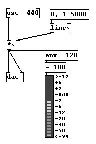
Then the VU shows changes in volume graphically. (VU is short for "volume").
In Pd-extended, you can also use the "pvu~" object for the VU meter conversion:

Another important thing: amplitudes above 1 and below -1 will be 'clipped'. If "dac~" sends the speaker a value outside the range of 1 to -1, the membrane simply stays at the furthest extreme.
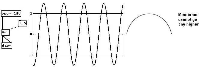
Increasing the volume of a sound to the point of 'clipping' results in an effect called overdrive.

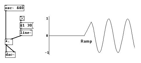
Another problem occurs when the speaker membrane has to span a large interval suddenly (e.g., when you turn on a sound); the result is a "click":

This is especially noticeable when the sound itself exhibits very smooth membrane movement, as with a sine tone. The "jolt" is easy to see in this illustration:

A "jolt" is usually a movement that is faster than 30 ms. To avoid this click, therefore, you need to build what's called a "ramp", i.e., a very fast crescendo at the beginning and end:
In Pd, you can also set membrane position for a sound wave where it should begin (or where it should jump to). This is called the phase of a wave. You can set the phase in Pd in the right inlet of the "osc~" object with numbers between 0 and 1:
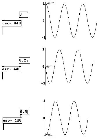
A wave's entire period is encompassed by the range from 0 to 1. However, it is often spoken of in terms of degrees, where the entire period has 360 degrees. One speaks, for example, of a "90 degree phase shift". In Pd, the input for the phase would be 0.25.
A phase shift doesn't have much effect on what we hear. We'll return to this concept later, however.
Let's say you have these two oscillators:

... and you connect them to "dac~". You'd get this:

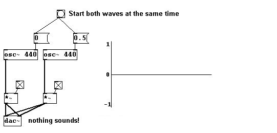
Due to the multiplicative factor, the individual waves only go from -0.5 to 0.5. Taken together, however, they cover a range from -1 to 1 and have a more complex form. This is because sound waves are additive. Simply stated: all vibrations occur in the same air. This additive quality also entails cancellations. Opposed waves, where one is "moving backwards" while the other is "moving forwards" cancel one another out. This is what happens when vibrations that have the same frequency are 180 degrees out of phase:
When many sound sources are involved, we usually have to multiply the total sound by a suitable factor to avoid exceeding the limits of 1 and -1:
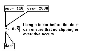
In this case, both oscillators are simply attached to a multiplication object. This automatically adds them (whenever several signals are given to an object as input, they are first added, then processed according to the object) before carrying out the multiplication.
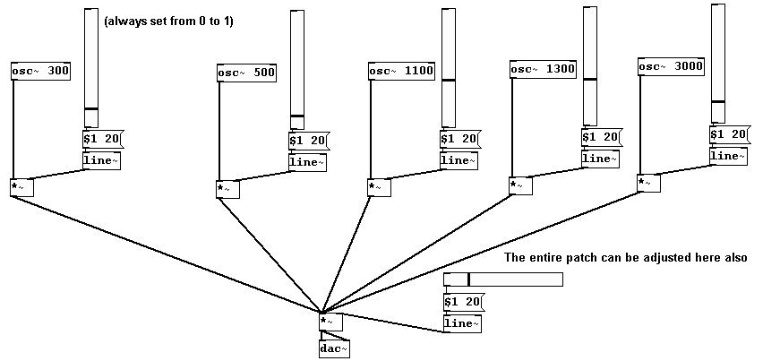
To create a chord with variable volume for every tone in the chord:
Glissandi that fade in and out smoothly at the beginning and end:
patches/3-1-2-2-2-glissandi-dim.pd

Say something into a microphone and play it back at a changed volume:
patches/3-1-2-2-3-edit-input.pd

Let's get 'symphonic': why not use 20 oscillators at once?
patches/3-1-2-2-4-oscillatorconcert1.pd
First make the subpatch "o1":

...make multiple copies...

...then turn them all on!
Of course, the parameters for each oscillator can be adjusted – and you've really got something to play with:
patches/3-1-2-2-4-oscillatorconcert2.pd
The speed of sound at 20 degrees Celsius (68 degrees Fahrenheit) is about 343 meters per second. You can calculate the length of a period in space and then check the result immediately...
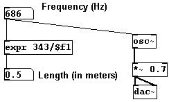
...by moving your head half a meter back and forth while listening to a frequency of 686 Hertz: you can clearly hear the wave's peak and its trough.
Several of the objects covered in Chapter 2 also have a version with a tilde. They work the same way, except that they work with signals instead of control data:
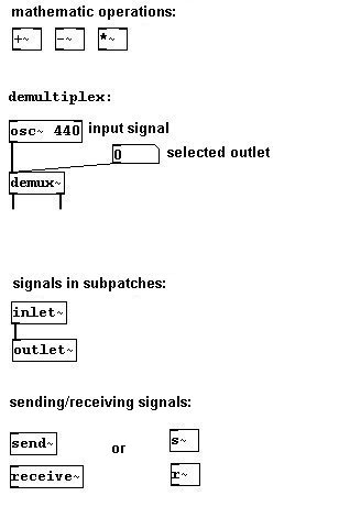
You can use "send~" with as many "receive~" objects as you like; however, you can only use one "send~" object:

You could also channel many different signals to one central location (for example, to the "dac~") by using "throw~" and "catch~":

Bit depth is also an important concept in Pd. The computer's processor only works with binary code, i.e., with 0 and 1. The bit number shows how many places are used for zeroes or ones. If you have only two places, you could make 22, that is, 4 different combinations:
       0 0
       0 1
       1 1
       1 0
The more places there are, the more detailed something can be processed. For Pd, which uses numbers to calculate frequencies, amplitude, etc., this means that the numbers can be processed more precisely, i.e., more decimal places can be used. Pd normally works with 16 bit, which is the quality of an audio CD. 16 bit means 216 = 65,536 possible values for each sample.
Volume and more importantly increments of volume are - in both objective and subjective terms - heavily influenced by factors like architectural characteristics of the room, age of the listener, etc. There is no single, precise form of measurement for volume, though there are theories of sound pressure and sound intensity. For more information, it is strongly recommended that you consult a book about acoustics.
You may have noticed that for significant parts of sound production in Pd two different units are used: frequency and MIDI numbers for pitch, root mean square and deciBel for amplitude, and milliseconds and samples for time.
For the last of these, the example of using "line~" to create a crescendo/decrescendo given under section 3.1.2.1.1. should be explained further:
If you were to use a "line" object (without a tilde) for this, it would likely result in undesired popping or clipping sounds. This would require two different units of time measurement to be combined; the problem is they are not synchronized. The different numeric intervals will likely not match up, which would cause irregularities in the form of short delays or even popping sounds to occur.
As described in Chapter 2.2.3.3.2, "line" generates a value every 20 milliseconds. That means it may not coincide with the samples. Though a new sample comes every 0.02 milliseconds, a "line" value may not coincide with a more or less simultaneous sample, which could lead to complications. A "line~" object (with tilde), however, generates a signal with 44100 values per second. These 44100 values are generated at precisely the same time as any another tilde object; they are always synchronized. The computer always processes 44100 samples per second synchronously regardless of their position in the patch.
| | ||
| 2.2 The control level | Home | 3.2 Additive Synthesis |