| 3.4 Sampling | ||
|---|---|---|
| Chapter 3. Audio | | |
| 3.4 Sampling | ||
|---|---|---|
| Chapter 3. Audio | | |
Let's clear up a potentially problematic issue to avoid any confusion: you've already learned that a sample is the smallest unit used for measuring and generating sound in a computer. The word 'sample' unfortunately also has another, quite different meaning in electronic music; it means a smallish section (usually a couple seconds long) of recorded sound. This chapter deals with the processing of short recorded bits of sound. First you'll have to learn how "array" works in Pd, which requires a fair amount of explanation.
There are various locations in the computer where files can be saved: main memory or hard disks. Access to main memory is very fast in comparison to the hard disk; however, it has much less available space.
In Pd you can save sound to both locations. Saving to the hard disk means that you are saving a fixed sound file. WAV or AIFF formats are typically used. Use the "writesf~" object to write a sound file to disk. The argument is the number of channels; this creates a corresponding number of inlets to which you attach the sounds you want to record. First you have to use the message "open [name]" to choose the name of the file you want to create. Start recording using "start" and stop it using "stop".

The other possible location is the main memory. Create one place for one sound using "array" (Put Array then click "ok"). It is also a visualization of the sound.
Let's first think of an array simply as storage for numbers. An array has a limited number of storage places. You can set this number using by right-clicking the array and going to "Properties". This opens two windows: one labeled "array" and the other labeled "canvas". In the "array" window, you can set the size. This number means the number of storage places. One number can be stored in each storage place.
You can allocate these cells using "tabwrite". The right argument determines the position; the left determines the value you want to save (as always: from right to left). In the array, the x-axis shows position and the y-axis shows the value:

You can use "array" to represent functions:
patches/3-4-1-1-2-function1.pd

Or without temporal stretching (if the example shown causes a stack overflow, inserting "del 0" between "spigot" and "f" will help):
patches/3-4-1-1-2-function2.pd

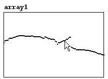
You could also draw in the array itself with the mouse, 'by hand' so to speak. If you move the mouse to a value in the array, the cursor (shaped like an arrow) will change its direction and you can draw by moving the mouse with the mouse button held.
Under 'Properties' (right-click on the array), you can set the following:

In the "array" window:
Name: Like all names in Pd, use alphanumeric characters without spaces, not only numbers.
Size: As described above.
"save contents": When checked, all values in an array will be saved. If you use large arrays or a large number of arrays, this could cause your patch to load very slowly.
"draw as points" / "polygon" / "bezier curve": Different kinds of visualization.
"delete me": When checked, this deletes the array! The empty box remains, however, and must also be deleted.
"view list": This displays all values in a list.
In the "canvas" window:
"graph on parent": This will be discussed later in 3.1.1.2.
X range: You can set the range for the x-axis here.
Y range: You can set the range for the y-axis here. Values that fall outside this range will also be saved, but this will enlarge the entire window so that these values can be seen.
"size": Visual size in the patch.
An array can also receive messages and "sends".
Renaming:

Making all values equal:

Changing the size:

The size can also be printed out:

Writing the contents to a text file:

Reading a text file:

You can also enter values like this. The first number determines which storage place to start with; all other values are for the positions thereafter:

You can also create hash marks on the axes and label them:

You can also number them:

First, the position is labeled; second, the numbers you want to display.
N.B.: Lines and labels are not stored in the patch, so you have to reenter them every time you open the patch.
You can, of course, also store sound in an array. For a computer, sound is - as has been often mentioned - nothing but a string of numbers, 44100 numbers to be precise. You could store one second of sound in an array; you'd just need to use 44100 storage places. Here's where the "tabwrite~" object comes into play. It receives the sound input and otherwise just a bang. Unlike with "tabwrite" (without a tilde) where you entered the storage place in the right inlet 'by hand' and the corresponding value on the left, when "tabwrite~" receives a "bang", it automatically starts with the first storage place and then proceeds at sample speed (44100 samples/sec). At the same time, every place is allocated a value received by the left inlet from the current sound, resulting in a total of 44100 stored numbers. Any sound that follows is not stored. If you want to stop prematurely, you can send a "stop" message.
patches/3-4-1-1-2-normalize.pd

If "tabwrite~" receives a float message, this number is interpreted as a sample offset. In other words, the sample that corresponds to this float number will be the starting point for the array.
One useful function is that it's possible to raise the overall volume after the fact. If, for example, the original recording is too quiet (i.e., the membrane of the microphone didn't vibrate especially strongly, which resulted in fairly small values), you can amplify it. This is called "normalizing". For this, you can use the following message:

You can also make a connection between sound files located in the main memory and those located on the hard disk in array. This is achieved with the "soundfiler" object. This object allows you to load a sound file stored on the hard disk into an array, or to save the contents of an array on the hard disk as a sound file. The command "read" is used to load a sound file. The arguments for the command are the name of the file (with the path if necessary) and then the name of the array to which you want to write.
patches/3-4-1-1-2-load-soundfile.pd

Once the file has successfully loaded, the size of the sound file in samples will be sent out the "soundfiler" object's outlet.
You can also include other commands (called "flags") in the message:

The resize command changes the array's size to match that of the sample (this is limited to 4000000 samples - about 90 seconds, though this can be changed with "maxsize").
Conversely, the command "write" saves the contents of an array as a sound file to the hard disk. In this case, the format (WAV or AIFF) must be given as a flag, then the name (with path designation if necessary) of the file you want to create, and then the name of the array.

Other important "flags" in this context are:
normalize: Optimizes a file's amplitude levels, as explained previously.
rate: Used to set the sample rate for a file.
As an alternative to array, you could also use "table". Create a "table" object; enter the name for the first argument and the size in samples for the second. This will create an array in a subpatch (click on the object in execute mode) that is treated like a normal array. This approach has the following advantage: the graphics for a normal array can be very complex. You can notice this when you move a big array around on the canvas: it moves very slowly. But if the graphic representation of an array is in a subpatch, the object itself can be moved much more easily.

Sound files that are on an external storage device like a hard disk can be read - that is, played back - in Pd with "readsf~". As with "writesf~", you use the messages "start" and "stop" (you could also use "1" and "0"). Enter the number of channels as the argument. The rightmost output sends a bang when the end of a file is reached.

Let's look at the control level for 'array': let's say you have an array with 10 storage places. You can use "tabread" to read every one of these places:
patches/3-4-1-2-read-array1.pd

The principle is basically the same for signals, except that you have to receive the saved values at a rate of 44100 numbers per second. That's why there is "tabread~". If you want to, say, play a sound stored in an array that lasts 1.5 seconds (= 66150 samples), you have to read the array values from 0 to 66149 at a rate of 44100 values a second. You can do this with "line~":
patches/3-4-1-2-read-array2.pd

"tabread~" receives the array name as an argument. You could also set the array you want to read with the message "set [arrayname]".
Now you can start to play with these values. For example, you could play it back in twice the time:

This cuts the playback speed in half. This causes everything to sound an octave lower because the time stretching makes all the soundwaves twice as long, which means their frequencies will be cut in half and thus sound an octave lower.
This leads the problem that every single sample you use needs to be played twice or else there will be gaps. To avoid this problem, there is a modified form of the "tabread~" object called "tabread4~", which interpolates intermediate values that it generates using information from the values that ultimately precede and follow it. (More specific information on this function is available at 3.4.4.) In most cases, "tabread4~" is more suitable for reading arrays. This requires a readout spectrum from 1 to n - 2, where 'n' is the size of the array you want to read.
Of course, you could also play something back faster, which would raise the frequency:

Later, when granular synthesis is explained, you'll learn how to alter tempo and pitch independently.
Playing a sample backwards is naturally also a possibility:

You could also use the "phasor~" object:

"phasor~" generates a series of numbers between 0 and 1 as a signal. If you multiply these values by 66148, you get a series of numbers from 0 to 66148. Enter 0.75 for the frequency so that the series occurs in exactly 1.5 seconds.
Another possibility would be to create your own array for the arrangement of the readout and use it to play back the first array:
patches/3-4-1-2-read-array3.pd

Or you could use an array to control the amplitude:

Or to control the frequency:

Once again you can see: we're using only numbers to control various parameters.
You can use as many "tabread~" objects as you like to read from the same array. However, you should never use two arrays with the same name, as it will almost certainly lead to errors.
In Chapter 2.2.3.1.2 we mentioned how numbers or series of numbers can be delayed. You can also do this with signals. This is done by creating a buffer into which signals are written and out of which signals are read following a certain delay. To create this buffer, you use a "delwrite~" object. The first argument is a freely chosen name; the second is the size in milliseconds. As input, give it the signal you want it to write in the buffer. Once the buffer is full, it is written over again from the beginning. If the buffer is 1000 milliseconds long, the last 1000 milliseconds of the incoming signal are stored in the buffer.
Use "delread~" to read from the buffer. The first argument is again the buffer name; the second is the delay (in milliseconds; can be changed using a control data entry in the input):

Logically the amount of delay in "delread~" must be smaller than or equal to the buffer size. If you have a delay of 2000 milliseconds but the buffer holds only 1000 milliseconds, it clearly won't work. Using a negative number for the delay interval is also impossible, as even Pd can't see into the future. You can use as many "delread~" objects as you like to read simultaneously from a delay buffer. You cannot look into the wave patterns in the buffer.
While you can change the delay interval in "delread~", you have to use a control data entry and there is a certain probability of error once you exceed a certain speed (this is again a conflict between control data and signals). For this reason, there is a special object for variable readings of delay buffers called "vd~" (short for "variable delay"). You give the delay interval (in milliseconds) as a signal as input and can change it however you like (though, again, you can't use negative numbers or exceed the buffer size):

"vd~", like "readsf4~", creates an interpolation.
Here's one way to pick out any position from a sample that you want:

If you change the graphic representation as described previously (2.2.4), then your patch could look like this:
patches/3-4-2-4-sampler-big.pd

Four canvas objects make up the colorful background of the sliders and array. N.B.: The graphics that were created last always appear on top of the other ones. Let's say you have "array1" and then you make a colored canvas object; you have to create "array1" once again (just copy and then delete the old one) so that it appears on top of the canvas object.
To explain exactly how this was done:
 |
And in the subpatch:

patches/3-4-2-5-loop-generator1.pd
 |
But with this loop generator, clicks occur. First, it is highly recommended that you put the array in a subpatch, because the graphic requires a lot of processing power. Second, on the loop's ends you should briefly go to 0 so that there is no sudden jump in value (which would cause a click). For this, you need to program "windowing". In sync with the readout of the array, this is determined in the amplitude by another array (here, "crown") that controls the dynamic envelope. This envelope has a value of zero at the beginning and end to ensure that there is no sudden change to the value when the loop repeats. Instead of the "crown" window, you could also use a "Hanning" window, which uses a part of the sine function (this will be covered later). Of course, the "crown" array should also be in another window as well, but it has been left this way for the sake of clarity.
 |
A simpler version of the loop can be created using feedback:
patches/3-4-2-5-loop-generator2.pd

A drawback to this is that there is a maximum loop duration; here it is 10000 milliseconds.
Or you can create a texture:

You have to be careful that the feedback doesn't 'explode', i.e., that its volume doesn't increase exponentially.
You can build a comb filter using audio delay. The idea is that you add the delay to the original signal. This results in amplifications and cancellations at regular intervals, which gives the spectrum the appearance of a comb:

If you know the frequency of a signal's fundamental, you can construct an octave doubler as follows: Let's take a wave...

...and this signal delayed by half the length of one period...

...adding them together gives you 0 (= cancellation). If you delay a periodic signal by the half the duration of one period and add it to the original, the fundamental tone (and all odd partials) is cancelled out. That would look like this:

But it doesn't quite work like that. You have to remember that Pd processes all audio data in blocks of 64 samples (unless you change the setting), because it is more efficient than individually processing each sample (cf. 3.1.1.3.2). With the above patch, you'd get a delay of 1,136 milliseconds, or 50 samples. You could alleviate this problem by using a buffer with a one-block delay (64 samples = 1,451 ms) to read the original; the same goes for the delay offset:

patches/3-4-2-9-oktavedoubler.pd
A special use of looping is the Karplus-Strong algorithm. It is one of the first examples of physical modeling synthesis, a process that attempts to replicate what occurs when a physical material vibrates. In our example, the physical model is a plucked string. When it is plucked, a string first vibrates chaotically then adjusts itself to the length of the string. It also loses energy, i.e., the vibration dies away. This can be reconstructed mathematically by taking an excerpt of white noise and playing it back periodically again and again by writing it to and reading it from a buffer:
patches/3-4-2-10-karplus-strong1.pd

The string effect can be enhanced if the material you start with vibrates more and more 'softly'. This works with by calculating the average: the average of every two samples is taken and this result is written to the buffer in place of the original values. The vibration becomes less and less 'angular'. Use the object "z~" (Pd-extended) to set the delay to one sample; enter the number of samples as the argument:
patches/3-4-2-10-karplus-strong2.pd

The tone is different every time. This is because "noise~" produces random numbers, which are naturally different every time. We could add the calculation for the resulting frequencies:

patches/3-4-2-10-karplus-strong3.pd
a) Build a record function into the sample player.
b) Create a patch for reverb or a texture with different delay times for the input signal, e.g., with multiples of the Fibonacci series (in which the next number is always the sum of the previous two: 0 1 1 2 3 5 8 13).
c) Use different Karplus-Strong sounds to make textures of varying densities.
d) Apply a comb filter to patches presented in the previous sections.
One way to simplify the combination of "tabread~" and a multiplied "phasor~" signal is "tabosc4~". This reads out an array for the frequency you enter. One limitation of this method is that the size of the array must be a power of two (e.g., 128, 512, 1024) plus three points (here, 1027 = 1024 + 3).
patches/3-4-3-1-arrayoscillator.pd

This touches on "wave shaping", a topic that will be further explained in chapter 3.5. You can draw any wave into an array using the mouse.
Yet another simplification is "tabplay~"; it simply plays an array back at the original speed (when banged). Conveniently, you can set the start and end points for playback (starting point and duration in samples):
patches/3-4-3-2-simply-play-array.pd

The "tabwrite~" and "tabread~" objects also have another special form: "tabsend~" and "tabreceive~". They write/read an array in sync with the "blocks" (3.1.1.3.2). "tabwrite~" writes each block in an array (of course, these must be the size of a block, which is set to 64 samples by default in Pd). "tabreceive~" reads the array in every block. We will return to this later in the chapter on FFT (3.8).
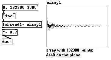
You know that you can play back an array at normal pitch or an octave higher, etc. But what if you want a glissando from the octave to the original pitch? For this, you'll need to subdivide into "main indicator" and "addition". The "main indicator" run at normal speed over the array. Let's use an array with 132300 points as an example, which equals 3000 milliseconds:
Then comes the "addition", which is what makes the glissando. Let's use a glissando that begins five chromatic steps above the original pitch and returns to the original pitch in 500 milliseconds. You need to make "line~" of this in reverse, then square the values:

Above this, you have to determine the factor for the frequencies of the five chromatic steps (cf. 3.1.1.4.3)...

...and finally conduct the following calculation:

This is the "addition" that is added to the "main indicator":
patches/3-4-3-4-sample-glissando1.pd

You can use any glissandi to the target pitch that you want; even negative values are possible:
patches/3-4-3-4-sample-glissando2.pd

Conversely, to move away from the original tone:
patches/3-4-3-4-sample-glissando3.pd

As a special function in Pd, you can create a sum of sine tones in an array - i.e., additive synthesis as described in Chapter 3.2. This is accomplished using the message "sinesum". The first argument is the (new) array size (should be a power of 2; three points will be added to this number automatically to ensure optimum connection of the beginning and ending of a phase) and also the volume factors for any number of partials:

Instead of sine waves, you could also use "cosinesum" to work with cosine waves.
Audio delay sometimes occurs when you don't want it to. You can even hear it when you have a microphone connected to a speaker and make an extremely short noise into the microphone, snapping your fingers, for example:

The sound card and especially the operating system determine the length of this "latency". Ideally the latency is so short (under 5 ms) that the human ear cannot perceive the delay. This requires a fast computer processor, a good sound card, and an appropriate operating system. You can set the latency under Media Audio settings:

In Microsoft Windows, you cannot at the present time (June 2008) achieve a latency of less than 50 ms without causing errors.
In this example you can see how "tabread4~" interpolation works:
patches/3-4-4-1-four-point-interpolation.pd

The jump from 1 to -1 is 'softened' by a kind of sinusoidal interpolation. As the name implies, four points are used and altered: namely the two directly in front of and the two directly behind the interval that you want to interpolate.
One way to delay something by a certain number of samples with "delread~" and "vd~" is by using a subpatch (otherwise the problem of block size, described previously in relation to octave displacement):
patches/3-4-4-2-samplewise-delay.pd


