| 3.8 Fourier analysis | ||
|---|---|---|
| Chapter 3. Audio | | |
| 3.8 Fourier analysis | ||
|---|---|---|
| Chapter 3. Audio | | |
Let's return to a basic concept of additive synthesis: a sound comprises partials. If you want to find out what the component parts of a sound are, you could employ a set of band-pass filters for every partial:
patches/3-8-1-1-analyze-partials.pd

This process performs what is called Fourier transformation. It divides the entire frequency spectrum into parts of equal size and determines the amplitude and phase for each part. One could in turn reconstruct the original signal from these values. The derivation of the component parts is called analysis; the reconstruction is called resynthesis. You can realize this using the objects "rfft~" and "irfft~":

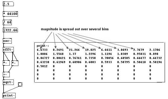
The size of the individual sections, called bins, is given by the block size. As discussed in Chapter 3.1.1.3.2, Pd always processes all tasks in blocks. Normally the block size in Pd is 64 samples. Using "print~" shows you all the values in a given block:
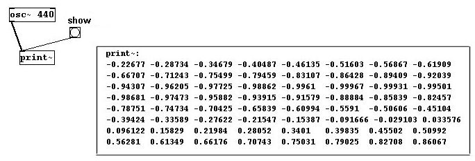
As with "snapshot~" or "unsig", you can see the amplitude values produced. With "print~" you can actually see ALL of the values generated, limited in number to one DSP block. Let's first stick to 64 samples; i.e., the entire spectrum up to 44100 Hertz is divided into bins with a size of 44100/64 = 689 Hz. The next thing we have to consider is that the amplitude and phase data with "FFT" is not represented in the customary format; they appear as sine and cosine values. For now, let's not pursue this particular facet in further detail; you can transform the data into a more readily comprehensible form as follows:
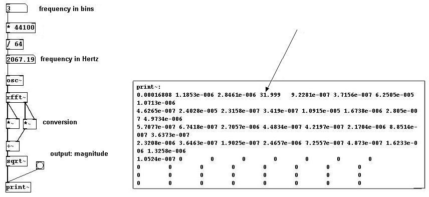
As you can see, "print~" generates 64 values for amplitude. The amplitude is given here as magnitude, always a positive value (because it was squared). Let's take a closer look: except for the third bin, which has a value of (ca.) 32, we have nothing but very small values. There is no calculation for numbers above the Nyquist frequency.
Usually a normalization process is conducted after a FFT process, because the amplitude values become fairly high. First, this is the block size:

You could present the FFT analysis in an array:
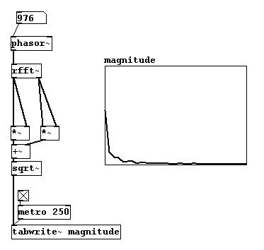
This way you can see the spectrum of a signal. N.B.: FFT turns information that occurs in time into information in frequencies; these are updated in every new block. One speaks of the time domain and the frequency domain.
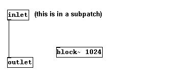
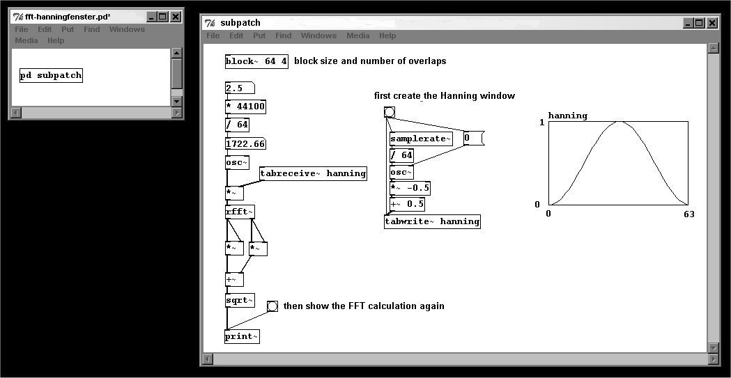
In Pd, the block size can only be changed in a subpatch. This is achieved using "block~":
When choosing the block size, be sure to consider that a larger block size allows you to work with lower frequencies. For example: with a size of 1024 samples, every bin is 44100/1024 = ~43 Hz in size, so you have a finer resolution. The downside is that the process takes longer.
Let's stick with a block size of 64 samples, which we can use to analyze the spectrum of a fundamental frequency of 689 Hz. But what if other frequencies occur in between?
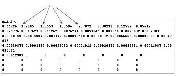
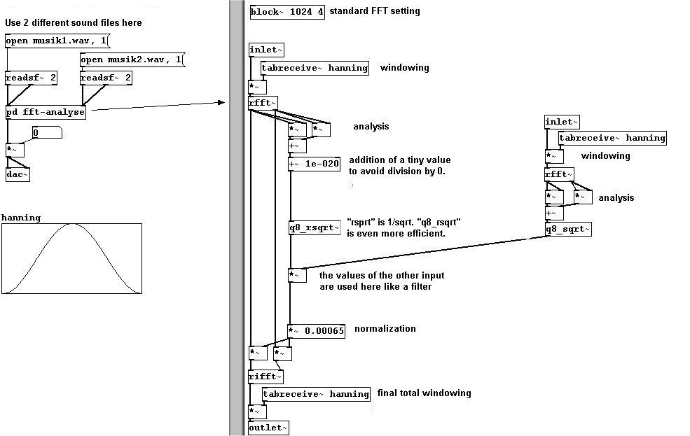
Then the information is divided among several bins and the phase changes with every analysis. This problem cannot be completely solved; you have to trick it a little bit. The normal way to solve the problem is to use overlapping windows as in granular synthesis; you create a windowed version of the original. You can use "tabreceive~" to achieve this, an object that always reads the given array in block size with a Hanning window - here with 64 samples.

This way, the magnitude values aren't so "spread out".
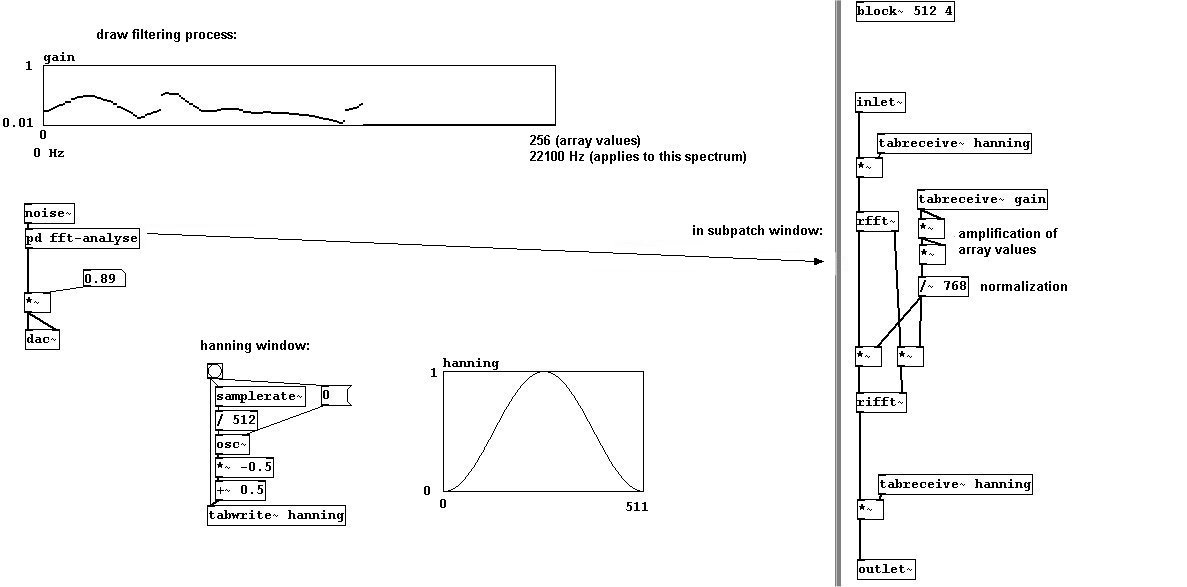
In addition to windowing, the windows need to overlap each other. This is very easy to do in Pd: simply enter the number of windows (usually 4) as the second argument of "block~". The result at the end also has to be windowed. The appropriate normalization for 4 overlapping windows is (3 * block size) / 2. Because you're using "block~", all of this has to fit in a subpatch.
patches/3-8-1-2-fft-subpatch.pd
By overlapping and windowing, the chances are good that a signal will be correctly analyzed.
What's useful about FFT, of course, is that the values it determines can be changed before you resynthesize the components into a sounding result. For example, you could set certain bins to be louder or quieter; you could build filters like high-pass, low-pass, etc., or 'draw' one yourself.
Convolution is a celebrated effect - folding a signal together with another; i.e., playing the average of their amplitudes. The Hanning calculation should be familiar to you by now. A block size of 1024 samples and four overlaps is standard.
patches/3-8-2-2-convolution.pd
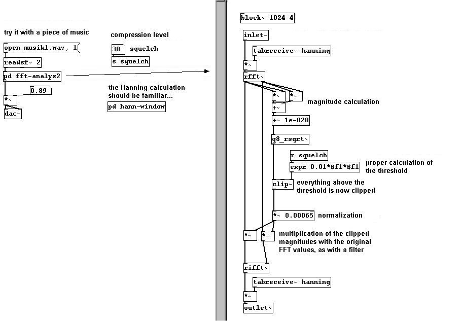
You could also build a compressor. This means that weaker volumes will be amplified a bit to bring them closer to the louder volumes. Simply use the magnitude values as factors for the outputs of "rfft", though be aware that values that exceed a certain threshold ("squelch") will simply be cut off at that point:
If you implement this in the folding of one of the two analyses, you get a richer convolution effect:

You can also play back certain bins with different amounts of delay to achieve what's called a "spectral delay". The FFT analysis is written to two different buffers. Using an array, you determine the delay for each bin. The maximum delay time is ca. 2500 milliseconds, as you have a buffer of 10000 milliseconds but 4 overlaps ("block~"), which means 10000/4 = 2500. To be precise, it's actually 2496 milliseconds: 2496 * 44.1 = ca. 110080 samples, which is 110080 / 512 = 215 possible bin positions. Since the input signal usually doesn't fit in the bin size, the values of the analysis are divided among several neighboring bins (cf. 3.8.1.2). If these neighboring bins occur at different times, there can be reductions in volume.
patches/3-8-2-4-spectral-delay.pd
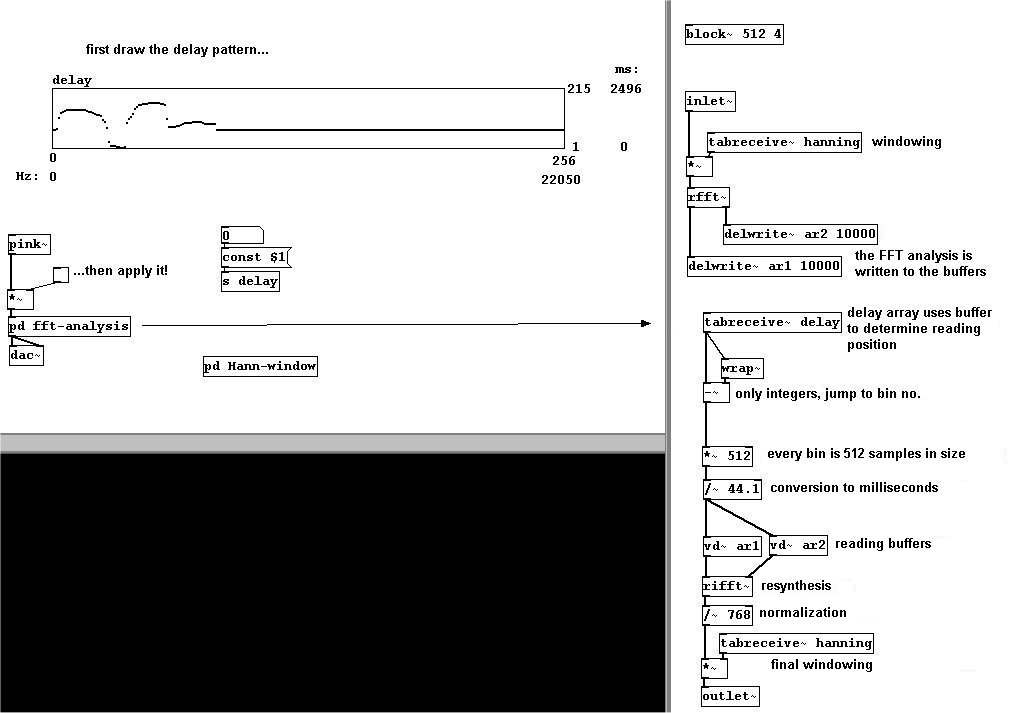
Try this out with a particularly eventful piece of music!
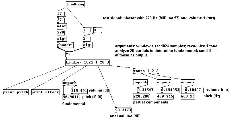
There is an object in Pd that is based on the FFT algorithm that performs an analysis of both volume AND pitch. It is called "fiddle~". It also determines the volumes and partials of the input signal.

The arguments it receives are: 1. Window size (in samples), 2. Number of tones to be recognized simultaneously (max. three different tones), 3. Number of peaks to find, and 4. Number of peaks to output. The default settings are: 1. 1024, 2. 1, 3. 20, 4. 0. As outputs (from left to right): 1. Pitch in MIDI (only when there is a change), 2. Volume in dB (only when there is an extreme change ("attack")), 3. Pitch and volume of the fundamental (as a list), 4. Total volume, and 5. Individual partials with their respective volumes (in Hertz / rms! - also as a list).
Messages for "fiddle~": to avoid constant data processing, you can turn off "auto mode" and activate "poll mode" instead; this only issues numbers when it gets a 'bang' message:

You can determine the window size (multiples of two):

Higher partials are not analyzed as intensively for determining the fundamental. You can change this, however, by instructing the object to analyze a certain partial at least half as intensely as the fundamental:
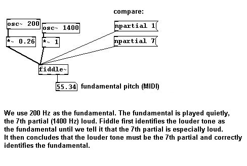
This is helpful if you know that certain partials of the input signal are especially strong (e.g., the third partial on a clarinet).
N.B.: The input signal is analyzed every half window size, i.e., if the window size is 1024, then 512 samples, which equals every 11.6 milliseconds. The smallest frequency that "fiddle~" can recognize is (44100 / window size) * 2.5; for a window size of 1024 samples, this is ca. 108 Hertz.
Here's one way to build a tuner:

For this visualization, an array with only one storage place was used.
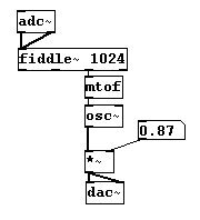
For the octave doubler described in 3.4.2.9, you can now use a microphone input as long as this fundamental can be used to conduct calculations (i.e., as long as the input signal is periodic and can be understood by "fiddle~"):
patches/3-8-3-3-oktavedoubler-fiddle.pd
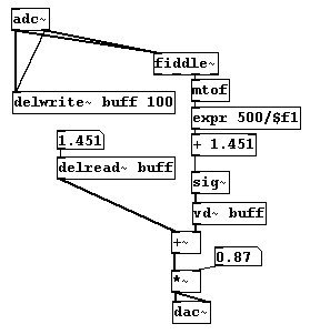
Many interesting applications can be imagined that use the "fiddle~" object in this way. A prototypical example would be a microphone input, like a singing voice, and to 'trace' the voice's melodic contour like a laser pointer:
The following dilemma arises: there is always a delay when using "fiddle~". The smaller the window size, the shorter this is. However, the smaller the window size, the higher the lowest range of pitches that can be recognized. Moreover, the result of "fiddle~" is always a bit chaotic. You can learn how to minimize this under 4.3.1.3